Polynomials

Polynomials constitute a rich class of functions which are both easy to describe and widely applicable in topics ranging from Fourier analysis, cryptography, and communication, to control and computational geometry. They show up in all sorts of EECS courses including 70’s sister courses 16A/16B, and then in the upper-division courses like 120, 123, etc. In this note, we will discuss some properties of polynomials which make them so useful. We will then describe how to take advantage of these properties to develop a secret sharing scheme.

Recall from your high school math that a polynomial in a single variable is of the form \(p(x) = a_d x^d + a_{d-1} x^{d-1} + \cdots + a_0\). Here the variable \(x\) and the coefficients \(a_i\) are usually real numbers. For example, \(p(x) = 5x^3 + 2x + 1\), is a polynomial of degree \(d = 3\). Its coefficients are \(a_3 = 5\), \(a_2 = 0\), \(a_1 = 2\), and \(a_0 = 1\). Polynomials have some remarkably simple, elegant, and powerful properties, which we will explore in this note.

First, a definition: we say that \(a\) is a root of the polynomial \(p(x)\) if \(p(a) = 0\). For example, the degree \(2\) polynomial \(p(x) = x^2 - 4\) has two roots, namely \(2\) and \(-2\), since \(p(2) = p(-2) = 0\). If we plot the polynomial \(p(x)\) in the \(x\)-\(y\) plane, then the roots of the polynomial are just the places where the curve crosses the \(x\) axis:

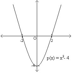
Notice that the graph goes through the \(x\)-axis at exactly two points, which are the roots (also known as \(x\)-intercepts). Another interesting fact about polynomials is that the sum of two degree \(d\) polynomials results in a polynomial of at most degree \(d\). For example, if \(p(x) = 3x^2 + 2x + 1\), and \(q(x) = 5x^2 + x + 4\), then \(p(x)\) and \(q(x)\) both have degree \(2\), and \(p(x) + q(x) = 8x2 + 3x + 5\), which is also a degree \(2\) polynomial. It is possible but unusual for the degree of the sum to decrease. (Take \(p(x) = x^2 + x + 1\) and \(q(x) = -x^2 + x + 1\). Both polynomials have degree \(2\), but \(p(x) + q(x) = 2x + 2\), which only has degree \(1\).) For this reason we will not explicitly focus on the case when the degree decreases unless it is fairly relevant to the explanation. You should keep this in mind as you read through this material. Now, we will discuss some very remarkable properties of polynomials and build powerful tools using only these simple and elegant facts.

We now state two fundamental properties of polynomials that we will prove in due course.

Property 1

A non-zero polynomial of degree \(d\) has at most \(d\) roots.

Property 2

Given \(d+1\) pairs \((x_1, y_1), \ldots, (x_{d+1}, y_{d+1})\), with all the \(x_i\) distinct, there is a unique polynomial \(p(x)\) of degree (at most) \(d\) such that \(p(x_i) = y_i\) for \(1 \leq i \leq d+1\).

Let us consider what these two properties say in the case that \(d =1\). A graph of a linear (degree \(1\)) polynomial \(y = a_1 x + a_0\) is a line. Property 1 says that if a line is not the \(x\)-axis (i.e. if the polynomial is not \(y = 0\)), then it can intersect the \(x\)-axis in at most one point.

Property 2 says that two points uniquely determine a line.

Polynomial Interpolation

Property 2 says that two points uniquely determine a degree \(1\) polynomial (a line), three points uniquely determine a degree \(2\) polynomial, four points uniquely determine a degree \(3\) polynomial, and so on. Given \(d+1\) pairs \((x_1, y_1), \ldots, (x_{d+1}, y_{d+1})\), how do we determine the polynomial \(p(x) = a_d x^d + \cdots + a_1 x + a_0\) such that \(p(x_i) = y_i\) for \(i = 1\) to \(d+1\)? We will give a very simple algorithm¹ for reconstructing the coefficients \(a_0, \ldots, a_d\), and therefore the polynomial \(p(x)\).

The method is called Lagrange interpolation: Let us start by solving an easier problem. Suppose that we are told that \(y_1 =1\) and \(y_j = 0\) for \(2 \leq j \leq d+1\). Now can we reconstruct \(p(x)\)? Yes, this is easy! Consider \(q(x) = (x - x_2)(x - x_3) \cdots (x-x_{d+1})\). This is a polynomial of degree \(d\) (the \(x_i\)’s are constants, and \(x\) appears \(d\) times). Also, we clearly have \(q(x_j) = 0\) for \(2 \leq j \leq d+1\). But what is \(q(x_1)\)? Well, \(q(x_1) = (x_1 - x_2)(x_1 - x_3) \cdots (x_1 - x_{d+1})\), which is some constant not equal to \(0\). Thus if we let \(p(x) = q(x)/q(x_1)\) (dividing is ok since \(q(x_1) \neq 0\)), we have the polynomial we are looking for. For example, suppose you were given the pairs \((1,1)\), \((2,0)\), and \((3,0)\). Then we can construct the degree \(d = 2\) polynomial \(p(x)\) by letting \(q(x) = (x - 2)(x - 3) = x^2 - 5x + 6\), and \(q(x_1) = q(1) = 2\). Thus, we can now construct \(p(x) = q(x)/q(x_1) = (x^2 - 5x + 6)/2\).

Of course the problem is no harder if we single out some arbitrary index \(i\) instead of \(1\): i.e. \(y_i = 1\) and \(y_j = 0\) for \(j \neq i\). Let us introduce some notation: let us denote by \(\Delta_i(x)\) the degree \(d\) polynomial that goes through these \(d+1\) points. Then \[\Delta_i(x) = \frac{\prod_{j\neq i} (x-x_j)}{\prod_{j\neq i} (x_i-x_j)}.\]

Let us now return to the original problem. Given \(d+1\) pairs \((x_1, y_1), \ldots, (x_{d+1}, y_{d+1})\), we first construct the \(d+1\) polynomials \(\Delta_{1}(x), \ldots , \Delta_{d+1}(x)\). Now we can write \(p(x) = \sum_{i = 1}^{d+1} y_i \Delta_i(x)\). Why does this work? First notice that \(p(x)\) is a polynomial of degree \(d\) as required, since it is the sum of polynomials of degree \(d\). And when it is evaluated at \(x_i\), \(d\) of the \(d+1\) terms in the sum evaluate to \(0\) and the \(i\)-th term evaluates to \(y_i\) times \(1\), as required.

As an example, suppose we want to find the degree-\(2\) polynomial \(p(x)\) that passes through the three points \((1,1)\), \((2,2)\) and \((3,4)\). The three polynomials \(\Delta_i\) are as follows: If \(d = 2\), and \(x_i = i\), for instance, then \[\begin{aligned} \Delta_1(x) &= \frac{(x - 2)(x - 3)}{(1 - 2)(1 - 3)} = \frac{(x - 2)(x - 3)}{2} = \frac{1}{2}x^2 - \frac{5}{2}x + 3;\\ \Delta_2(x) &= \frac{(x - 1)(x - 3)}{(2 - 1)(2 - 3)} = \frac{(x - 1)(x - 3)}{-1} = -x^2 +4x -3;\\ \Delta_3(x) &= \frac{(x - 1)(x - 2)}{(3 - 1)(3 - 2)} = \frac{(x - 1)(x - 2)}{2} = \frac{1}{2}x^2 -\frac{3}{2}x +1.\end{aligned}\] The polynomial \(p(x)\) is therefore given by \[p(x) = 1\cdot\Delta_1(x) + 2\cdot\Delta_2(x) + 4\cdot\Delta_3(x) = \frac{1}{2}x^2 -\frac{1}{2}x +1.\] You should verify that this polynomial does indeed pass through the above three points.

Proof of Property 2

We would like to prove Property 2.

We have shown how to find a polynomial \(p(x)\) such that \(p(x_i) = y_i\) for \(d+1\) pairs \((x_1,y_1),\dots,(x_{d+1},y_{d+1})\). This proves part of Property 2 (the existence of the polynomial). How do we prove the second part, that the polynomial is unique? Suppose for contradiction that there is another polynomial \(q(x)\) such that \(q(x_i) = y_i\) for all \(d+1\) pairs above. Now consider the polynomial \(r(x) = p(x) - q(x)\). Since we are assuming that \(q(x)\) and \(p(x)\) are different polynomials, \(r(x)\) must be a non-zero polynomial of degree at most \(d\). Therefore, Property 1 implies it can have at most \(d\) roots. But on the other hand \(r(x_i) = p(x_i) - q(x_i) = 0\) on \(d+1\) distinct points. Contradiction. Therefore, \(p(x)\) is the unique polynomial that satisfies the \(d+1\) conditions.

Polynomial Division

Let’s take a short digression to discuss polynomial division, which will be useful in the proof of Property 1. If we have a polynomial \(p(x)\) of degree \(d\), we can divide by a polynomial \(q(x)\) of degree \(\leq d\) by using elementary-school long division. The result will be: \[p(x) = q(x)q'(x) + r(x)\]

where \(q'(x)\) is the quotient and \(r(x)\) is the remainder. The degree of \(r(x)\) must be smaller than the degree of \(q(x)\).

Example. We wish to divide \(p(x) = x^3 + x^2 - 1\) by \(q(x) = x - 1\):

Now \(p(x) = x^3 + x^2 - 1 = (x-1)(x^2 + 2x + 2) + 1\), \(r(x) = 1\) and \(q'(x) = x^2 + 2x + 2\).

Proof of Property 1

Now let us turn to Property 1: a non-zero polynomial of degree \(d\) has at most \(d\) roots.The idea of the proof is as follows. We will prove the following claims:

Claim 1

If \(a\) is a root of a polynomial \(p(x)\) with degree \(d\), then \(p(x) = (x-a)q(x)\) for a polynomial \(q(x)\) with degree \(d-1\).

Claim 2

A polynomial \(p(x)\) of degree \(d\) with distinct roots \(a_1,\dots,a_d\) can be written as \(p(x) = c(x-a_1)\cdots(x-a_d)\).

Claim 2 implies Property 1. We must show that \(a \neq a_i\) for \(i = 1, \ldots d\) cannot be a root of \(p(x)\). But this follows from Claim 2, since \(p(a) = c(a-a_1)\cdots(a-a_d) \neq 0\).

Proof of Claim 1

Dividing \(p(x)\) by \((x-a)\) gives \(p(x) = (x-a)q(x) + r(x)\), where \(q(x)\) is the quotient and \(r(x)\) is the remainder. The degree of \(r(x)\) is necessarily smaller than the degree of the divisor \((x-a)\). Therefore \(r(x)\) must have degree \(0\) and therefore is some constant \(c\). But now substituting \(x=a\), we get \(p(a) = c\). But since \(a\) is a root, \(p(a) = 0\). Thus \(c= 0\) and therefore \(p(x) = (x-a)q(x)\), thus showing that \((x-a) \mid p(x)\).

Claim 1 Implies Claim 2

Proof by induction on \(d\).

• Base Case: We must show that a polynomial \(p(x)\) of degree 1 with root \(a_1\) can be written as \(p(x) = c(x-a_1)\). By Claim 1, we know that \(p(x) = (x-a_1)q(x)\), where \(q(x)\) has degree 0 and is therefore a constant.

• Inductive Hypothesis: A polynomial of degree \(d-1\) with distinct roots \(a_1,\dots,a_{d-1}\) can be written as \(p(x) = c(x-a_1)\cdots(x - a_{d-1})\).

• Inductive Step: Let \(p(x)\) be a polynomial of of degree \(d\) with distinct roots \(a_1,\cdots,a_d\). By Claim 1, \(p(x) = (x-a_d)q(x)\) for some polynomial \(q(x)\) of degree \(d-1\). Since \(0 = p(a_i) = (a_i-a_d)q(a_i)\) for all \(i\neq d\) and \(a_i-a_d \neq 0\) in this case, \(q(a_i)\) must be equal to 0. Then \(q(x)\) is a polynomial of degree \(d-1\) with distinct roots \(a_1,\dots,a_{d-1}\). We can now apply the inductive assumption to \(q(x)\) to write \(q(x) = c(x-a_1)\cdots(x - a_{d-1})\). Substituting in \(p(x) = (x-a_d)q(x)\), we finally obtain that \(p(x) = c(x-a_1)\cdots(x-a_d)\).

Finite Fields

Both Property 1 and Property 2 also hold when the values of the coefficients and the variable \(x\) are chosen from the complex numbers instead of the real numbers or even the rational numbers. The proofs² do not hold if the values are restricted to being natural numbers or integers. Let us try to understand this a little more closely. The only properties of numbers that we used in polynomial interpolation and in the proof of Property 1 is that we can add, subtract, multiply and divide any pair of numbers as long as we are not dividing by \(0\). We cannot subtract two natural numbers and guarantee that the result is a natural number. And dividing two integers does not usually result in an integer.

But if we work with numbers modulo a prime³ \(m\), then we can add, subtract, multiply and divide (by any non-zero number modulo \(m\)). To check this, recall that \(x\) has an inverse mod \(m\) if \(\gcd(m,x)=1\), so if \(m\) is prime all the numbers \(\{1,\ldots,m-1\}\) have an inverse mod \(m\). So both Property 1 and Property 2 hold if the coefficients and the variable \(x\) are restricted to take on values modulo \(m\). This remarkable fact that these properties hold even when we restrict ourselves to a finite set of values is the key to several applications that we will presently see.

Let us consider an example of degree \(d = 1\) polynomials modulo \(5\). Let \(p(x) = 2x + 3 \pmod 5\). The roots of this polynomial are all values \(x\) such that \(2x + 3 = 0 \pmod 5\) holds. Solving for \(x\), we get that \(2x = -3 = 2 \pmod 5\) or \(x = 1 \pmod 5\). Note that this is consistent with Property 1 since we got only 1 root of a degree 1 polynomial.

Now consider the polynomials \(p(x) = 2x + 3\) and \(q(x) = 3x-2\) with all numbers reduced mod \(5\). We can plot the value of each polynomial \(y\) as a function of \(x\) in the \(x\)-\(y\) plane. Since we are working modulo \(5\), there are only \(5\) possible choices for \(x\), and only \(5\) possible choices for \(y\):

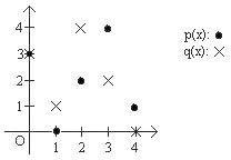
Notice that these two “lines" intersect in exactly one point, even though the picture looks nothing at all like lines in the Euclidean plane! Looking at these graphs it might seem remarkable that both Property 1 and Property 2 hold when we work modulo \(m\) for any prime number \(m\). But as we stated above, all that was required for the proofs of Property 1 and Property 2 was the ability to add, subtract, multiply and divide any pair of numbers (as long as we are not dividing by \(0\)), and they hold whenever we work modulo a prime \(m\).

When we work with numbers modulo a prime \(m\), we say that we are working over a finite field, denoted by \(\mathbb{F}_m\) or \(\operatorname{GF}(m)\) (for Galois Field). In order for a set to be called a field, it must satisfy certain axioms which are the building blocks that allow for these amazing properties and others to hold. If you would like to learn more about fields and the axioms they satisfy, you can visit Wikipedia’s site and read the article on fields: http://en.wikipedia.org/wiki/Field_%28mathematics%29. While you are there, you can also read the article on Galois Fields and learn more about some of their applications and elegant properties which will not be covered in this lecture: http://en.wikipedia.org/wiki/Galois_field. (Take Math 113 and Math 114 to really get into this stuff, or take EECS 229B which also covers many of these properties as it builds the fundamentals of error-correcting codes.)

If you are interested in learning more about fields or finite fields, you can look up a standard book on “Abstract Algebra” or look up wikipedia. In a nutshell, in order for a set to be called a field, it must have addition and multiplication operations defined on the set and must also satisfy certain axioms:

• Closure under addition and multiplication

• Associativity of addition and multiplication

• Commutativity of addition and multiplication

• Existence of additive and multiplicative identity elements

• Existence of additive inverses and multiplicative inverses

• Distributivity of multiplication and addition

These axioms imply that a field is also associated with subtraction and division operators. Since these are the operations we rely on in the proofs above, we can view field axioms as the building blocks which allow for these amazing properties and others to hold.

Natural numbers or integers do not satisfy the field axioms. For example, the multiplicative inverse of a natural number is generally not a natural number (i.e. is there a natural number \(x\) such that \(5\cdot x = 1\)?). On the other hand, complex, real and rational numbers do constitute fields – and therefore properties 1 and 2 hold as well. The field \(\operatorname{GF}(m)\) is especially interesting as it is finite. This property will lead to its applicability in several settings, as we will see in the next two sections.

Counting

How many polynomials of degree (at most) \(2\) are there modulo \(m\)? This is easy: there are \(3\) coefficients, each of which can take on one of \(m\) values for a total of \(m^3\). Writing \(p(x) = a_d x^d + a_{d-1} x^{d-1} + \cdots + a_0\) by specifying its \(d+1\) coefficients \(a_i\) is known as the coefficient representation of \(p(x)\). Is there any other way to specify \(p(x)\)?

Sure, there is! Our polynomial of degree (at most) \(2\) is uniquely specified by its values at any three points, say \(x = 0, 1, 2\). Once again each of these three values can take on one of \(m\) values, for a total of \(m^3\) possibilities. In general, we can specify a degree \(d\) polynomial \(p(x)\) by specifying its values at \(d+1\) points, say \(0, 1, \ldots , d\). These \(d+1\) values, \((y_0,y_1, \dots,y_d)\) are called the value representation of \(p(x)\). The coefficient representation can be converted to the value representation by evaluating the polynomial at \(0, 1, \dots, d\). And as we’ve seen, Lagrange interpolation can convert the value representation to the coefficient representation.

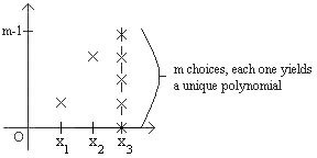
So if we are given three pairs \((x_1, y_1), (x_2,y_2), (x_3, y_3)\) then there is a unique polynomial of degree \(2\) such that \(p(x_i) = y_i\). But now, suppose we were only given two pairs \((x_1, y_1), (x_2, y_2)\); how many distinct degree \(2\) polynomials are there that go through these two points? Notice that there are exactly \(m\) choices for \(y_3\), and for each choice there is a unique (and distinct) polynomial of degree \(2\) that goes through the three points \((x_1, y_1), (x_2,y_2), (x_3, y_3)\). It follows that there are exactly \(m\) polynomials of degree at most \(2\) that go through \(2\) points \((x_1, y_1), (x_2, y_2)\), as shown below:

What if you were only given one point \((x_1, y_1)\)? Well, there are \(m^2\) choices for \(y_2\) and \(y_3\), yielding \(m^2\) polynomials of degree at most \(2\) that go through the point given. A pattern begins to emerge, as is summarized in the following table:

\[\begin{array}{|c|} \hline \text{polynomials of degree } \le d \text{ over } \mathbb{F}_m \\ \hline \begin{array}{c|c} \text{number of points} & \text{number of polynomials} \\ \hline d + 1 & 1 \\ d & m \\ d - 1 & m^2 \\ \vdots & \vdots \\ d - k & m^{k+1} \\ \vdots & \vdots \\ 0 & m^{d+1} \end{array} \\ \hline \end{array}\]

Note that the reason that we can count the number of polynomials in this setting is because we are working over a finite field. If we were working over an infinite field such as the rationals, there would be infinitely many polynomials of degree \(d\) that can go through \(d\) points! Think of a line, which has degree one. If you were just given one point, there would be infinitely many possibilities for the second point, each of which uniquely defines a line.

Here we are using the standard coefficient representation of a degree \(d\) polynomial. The properties we discussed in the previous sections illustrate that there are two ways to write polynomials: a coefficient representation and a value representation. The coefficient representation of a degree \(d\) polynomial can be thought of as a string \((a_0,\dots,a_d)\) of length \(d+1\), where the polynomial is equal to \(a_dx^d + a_{d-1}x^{d-1} + \cdots + a_0\) and each \(a_i\) is an element of \(\operatorname{GF}(q)\). The value representation can also be thought of as a string \((y_0,\dots,y_d)\) of length \(d+1\), which we interpret as the values of the polynomial at fixed points \(x_0,\dots,x_d\in \operatorname{GF}(q)\). As we’ve seen, polynomial interpolation can convert the value representation to the coefficient representation. The coefficient representation can be converted to the value representation by evaluating the polynomial at \(x_0,\dotsc, x_d\).

What happens if only part of either of these representations is specified? For example, what if we are given only \(k\) coefficients instead of \(d+1\)? Then there are \(d+1-k\) coefficients left to choose, and no matter which coefficients we choose, we will end up with a polynomial. Therefore, \(k\) coefficients specify a class of up to \(q^{d+1-k}\) polynomials. The same applies in the value representation, since we are again representing the polynomial by a string of elements in \(\operatorname{GF}(q)\). This symmetry is crucial to applications such as secret sharing, which we will see blow.

Secret Sharing

In the late 1950’s and into the 1960’s, during the Cold War, President Dwight D. Eisenhower approved instructions and authorized top commanding officers for the use of nuclear weapons under very urgent emergency conditions. Such measures were set up in order to defend the United States in case of an attack in which there was not enough time to confer with the President and decide on an appropriate response. This would allow for a rapid response in case of a Soviet attack on U.S. soil. This is a perfect situation in which a secret sharing scheme could be used to ensure that a certain number of officials must come together in order to successfully launch a nuclear strike, so that for example no single person has the power and control over such a devastating and destructive weapon. Suppose the U.S.  government finally decides that a nuclear strike can be initiated only if at least \(k > 1\) major officials agree to it. We want to devise a scheme such that (1) any group of \(k\) of these officials can pool their information to figure out the launch code and initiate the strike but (2) no group of \(k - 1\) or fewer have any information about the launch code, even if they pool their knowledge. For example, they should not learn whether the secret is odd or even, a prime number, divisible by some number \(a\), or the secret’s least significant bit. How can we accomplish this?

Suppose that there are \(n\) officials indexed from \(1\) to \(n\) and the launch code is some natural number \(s\). Let \(q\) be a prime number larger than \(n\) and \(s\). We will work over \(\operatorname{GF}(q)\) from now on.

Now pick a random polynomial \(P(x)\) of degree \(k - 1\) such that \(P(0) = s\) and give \(P(1)\) to the first official, \(P(2)\) to the second,…, \(P(n)\) to the \(n^{\text{th}}\). Then

• Any \(k\) officials, having the values of the polynomial at \(k\) points, can use Lagrange interpolation to find \(P\), and once they know what \(P\) is, they can compute \(P(0) = s\) to learn the secret. Another way to say this is that any \(k\) officials have between them a value representation of the polynomial, which they can convert to the coefficient representation, which allows them to evaluate \(P(0) = s\).

• Any group of \(k - 1\) officials has no information about \(s\). So they know only \(k-1\) points through which \(P(x)\), an unknown polynomial of degree \(k-1\) passes. They wish to reconstruct \(P(0)\). But by our discussion in the previous section, for each possible value \(P(0) = b\), there is a unique polynomial of degree \(k-1\) that passes through the \(k-1\) points of the \(k-1\) officials as well as through \((0, b)\). Hence the secret could be any of the \(q\) possible values \(\{0,1,\ldots,q-1\}\), so the officials have — in a very precise sense — no information about \(s\). Another way of saying this is that the information of the officials is consistent with \(q\) different value representations, one for each possible value of the secret, and thus the officials have no information⁴ about \(s\).

Example. Suppose you are in charge of setting up a secret sharing scheme, with secret \(s=1\), where you want to distribute \(n = 5\) shares to \(5\) people such that any \(k = 3\) or more people can figure out the secret, but two or fewer cannot. Let’s say we are working over \(\operatorname{GF}(7)\) (note that \(7>s\) and \(7>n\)) and you randomly choose the following polynomial of degree \(k-1 = 2\): \(P(x) = 3x^2 + 5x + 1\) (here, \(P(0) = 1 = s\), the secret). So you know everything there is to know about the secret and the polynomial, but what about the people that receive the shares? Well, the shares handed out are \(P(1) = 2\) to the first official, \(P(2) = 2\) to the second, \(P(3) = 1\) to the third, \(P(4) = 6\) to the fourth, and \(P(5) = 3\) to the fifth official. Let’s say that officials \(3\), \(4\), and \(5\) get together (we expect them to be able to recover the secret). Using Lagrange interpolation, they compute the following delta functions: \[\begin{aligned} \Delta_3(x) &= \frac{(x - 4)(x - 5)}{(3 - 4)(3 - 5)} = \frac{(x - 4)(x - 5)}{2} = 4(x-4)(x-5);\\ \Delta_4(x) &= \frac{(x - 3)(x - 5)}{(4 - 3)(4 - 5)} = \frac{(x - 3)(x - 5)}{-1} = 6(x-3)(x-5);\\ \Delta_5(x) &= \frac{(x - 3)(x - 4)}{(5 - 3)(5 - 4)} = \frac{(x - 3)(x - 4)}{2} = 4(x-3)(x-4).\end{aligned}\] They then compute the polynomial over \(\operatorname{GF}(7)\): \(P(x) = (1)\Delta_3(x)+(6)\Delta_4(x)+(3)\Delta_5(x) = 3x^2+5x+1\) (verify the computation!). Now they simply compute \(P(0)\) and discover that the secret is \(1\).

Let’s see what happens if two officials try to get together, say persons \(1\) and \(5\). They both know that the polynomial looks like \(P(x) = a_2x^2 + a_1x + s\). They also know the following equations: \[\begin{aligned} P(1) &= a_2 + a_1 + s = 2\\ P(5) &= 4a_2 + 5a_1 + s = 3\end{aligned}\] But that is all they have two equations with three unknowns, and thus they cannot find out the secret. This is the case no matter which two officials get together. Notice that since we are working over \(\operatorname{GF}(7)\), the two people could have guessed the secret (\(0 \le s \le 6\)) and constructed a unique degree 2 polynomial (by Property 2). But the two people combined have the same chance of guessing what the secret is as they do individually. This is important, as it implies that two people have no more information about the secret than one person does.